Web URL Scraping: Designing a High-Throughput URL Crawler with Efficient Storage

Web scraping at scale presents significant challenges, especially when dealing with millions of hyperlinks per request and handling 10,000+ requests per minute. The system must efficiently crawl web pages, extract hyperlinks recursively, and store them while ensuring high throughput, low latency, and minimal storage overhead.

In this blog, we will explore how to design a distributed web scraping system that supports the following functionalities:

• A POST API to accept a list of URLs, start a web scraping job, and return a job_id.

• A GET API to return the job progress percentage and, when completed, the full list of scraped URLs.

We will analyze system constraints, traffic implications, and various buffering strategies before writing data to long-term storage.

Functional Requirements

1. POST API (/scrape)

   • Accepts a list of URLs to crawl.

   • Extracts hyperlinks recursively until no new links are found.

   • Returns a unique job_id for tracking progress.

   {
       "urls": ["https://example.com", "https://example.org"]
   }
   

   Response:

   {
       "job_id": "abc123"
   }
   

2. GET API (/status/{job_id})

   • Returns the progress of the scraping job.

   • Once complete, provides access to the full list of scraped URLs.

     
     Response(In Progress)

     {
         "job_id": "abc123",
         "status": "in_progress",
         "progress": 65,
         "urls_scraped": 650000,
         "total_urls": 1000000
     }            

     Response(Completed)

{
    "job_id": "abc123",
    "status": "completed",
    "urls": ["https://example.com", "https://example.com/page1", "..."]
}
      

Non-Functional Requirements

• Scalability → Must handle 10,000+ requests per minute.

• High Throughput → Each URL may contain millions of hyperlinks.

• Fault Tolerance → Should handle failures and retry failed URLs.

• Storage Efficiency → Store billions of URLs while minimizing storage costs.

• Real-Time Progress Tracking → Provide job status updates with minimal overhead.

System Constraints and Traffic Analysis

1. URL Growth Rate

Each URL may contain multiple hyperlinks, leading to exponential growth in the number of URLs processed. If each URL contains 1 million hyperlinks and we recursively scrape them:

Level 0 (Initial URLs): 1,000  
Level 1 (1M per URL): 1,000 × 1M = 1B  
Level 2 (1M per new URL): 1B × 1M = 1T (trillion!)  

To prevent infinite expansion, limits must be placed on recursion depth and duplicate URL processing.

2. Storage Estimation

Assuming each URL is 100 bytes, storing 1 billion URLs per request requires:

1B × 100 bytes = 100 GB per request

At 10,000 requests per minute, the system could generate:

10,000 × 100 GB = 1 PB per minute

To handle this load efficiently, compression, partitioning, and deduplication are necessary.

3. Read/Write Traffic Considerations

Given the high ingestion rate, the system should:

• Support high-throughput writes to prevent bottlenecks.

• Ensure low-latency reads when retrieving job progress or results.

• Batch writes to minimize API calls to storage systems like Amazon S3.

High-Level Architecture

🔹 API Gateway → Manages request throttling and rate limits.
🔹 Distributed Scraper Workers → Process URLs concurrently.
🔹 URL Deduplication → Ensures we don’t scrape the same page multiple times.
🔹 Buffering Layer → Temporarily holds URLs before writing to S3.
🔹 Storage (Amazon S3 + Compressed text) → Efficiently stores billions of URLs.
🔹 Job Tracking (Redis/DB) → Tracks the progress of ongoing jobs.

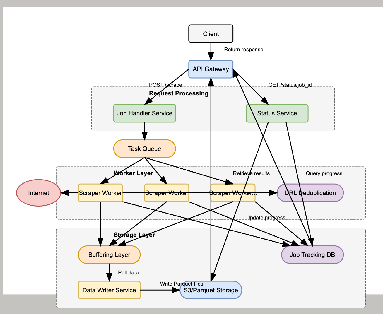
High-Level System Architecture

1. Components Overview

• API Gateway → Handles incoming requests and applies rate limits.

• Task Queue (Kafka/RabbitMQ) → Distributes scraping jobs to workers.

• Scraper Workers → Fetch and parse web pages concurrently.

• URL Deduplication Store (Redis/Bloom Filters) → Prevents re-scraping the same URLs.

• Buffering Layer → Stores URLs temporarily before writing to storage.

• Storage (Amazon S3/Compressed layer) → Long-term storage for scraped URLs.

• Job Tracking Database (PostgreSQL/DynamoDB/Redis) → Tracks job progress and completion.

2. Data Flow

1. Client submits a list of URLs via POST /scrape API.

2. The request is added to a distributed queue (e.g., Kafka, SQS).

3. Scraper workers fetch URLs, extract hyperlinks, and store them in a temporary buffer.

4. Buffers are periodically flushed to S3 to optimize storage writes.

5. The job progress is updated in a database for tracking.

6. The client queries GET /status/{job_id} to monitor the scraping job.

7. Once complete, the system provides a pre-signed S3 URL for downloading the results.

Storage Design and URL Buffering

1. Challenges of Writing URLs to S3

Since Amazon S3 does not support incremental writes, URLs must be batched and flushed efficiently. Writing each URL separately would lead to excessive API calls and high costs.

2. Buffering Strategies

To optimize writes, the system can use:

• Kafka → URLs are published to Kafka, consumed in batches, and written to S3.

• Redis Queue → URLs are pushed into Redis, periodically flushed in bulk.

• Kinesis Firehose → AWS-managed service that automatically buffers and writes to S3.

• In-Memory Buffers (Java/Python) → Simple approach but limited by system memory.

3. Efficient Storage & URL Buffering

🚀 Storage Challenges

📌 S3 Doesn’t Support Incremental Writes → Writing URLs one-by-one is expensive.
📌 Batching Strategies:

• Kafka → URLs are batched before writing.

• Redis Queue → Periodic bulk flush to S3.

• Kinesis Firehose → AWS-managed streaming storage.

📌 Recommended Storage Format → Compressed GZIP in Object Storage (S3)
🔹 Batch Size: 100,000 - 1,000,000 URLs per file
🔹 Compression: GZIP (space-efficient, fast reads)
🔹 File Naming: s3://scraper-results/{job_id}/part-{batch_number}.gzip
🔹 Parallel Writes: Multiple workers write partitions concurrently.

Comparison of Storage Architectures: Block, File, and Object Storage

When choosing the right storage system for a large-scale web scraping solution, understanding the file size limits, scalability, and storage constraints is critical. Below is an in-depth comparison of Block Storage, File Storage, and Object Storage, highlighting their limitations.

---

1. Block Storage

📌 How It Works:

• Data is divided into fixed-sized blocks and stored across physical or virtual disks.

• Block storage is used in Amazon EBS (Elastic Block Store), SAN (Storage Area Network), and iSCSI disks.

📌 Limits & Constraints:

• Maximum File Size: 16 TiB per volume (AWS EBS GP3)

• Maximum Storage Capacity: 64 TiB per instance (EBS Multi-Attach Mode)

• Limited Scalability: Requires manual volume provisioning & cannot scale infinitely.

• Throughput Limits: IOPS-based → Higher throughput requires expensive high-IOPS SSDs.

• Latency: Low (~ms level latency) for high-performance applications.

📌 Best Use Cases:
✅ Databases (MySQL, PostgreSQL, MongoDB)
✅ High-performance applications (Virtual Machines, Kubernetes StatefulSets)

---

2. File Storage

📌 How It Works:

• Organizes data in hierarchical directories & files using NFS (Network File System) or SMB (Server Message Block).

• Common examples: AWS EFS (Elastic File System), Google Filestore, traditional NAS systems.

📌 Limits & Constraints:

• Maximum File Size: 47.9 TiB per file (AWS EFS)

• Maximum Storage Capacity: Petabyte-scale (AWS EFS scales up automatically)

• Performance Bottlenecks: As file count grows into billions, metadata indexing slows down retrieval.

• Latency: Higher (~ms to seconds) compared to block storage due to file system overhead.

• Concurrency Limit: 100s-1000s of clients accessing a shared file system can lead to contention.

📌 Best Use Cases:
✅ Shared enterprise file systems (collaborative environments, engineering design files, log storage)
✅ Media storage (video processing, machine learning datasets)

---

3. Object Storage (Recommended for Large-Scale URL Scraping)

📌 How It Works:

• Stores data as objects in a flat namespace with metadata and unique identifiers.

• Common solutions: Amazon S3, Google Cloud Storage, MinIO, Azure Blob Storage.

📌 Limits & Constraints:

• Maximum File Size: 5 TiB per object (Amazon S3)

• Maximum Storage Capacity: Unlimited (Amazon S3 scales infinitely)

• Write Constraints: Objects cannot be modified incrementally; updates require overwriting the entire object.

• Performance Bottlenecks: Higher read latency (~100ms) than block/file storage.

• Concurrency: Supports millions of requests per second (designed for high throughput).

📌 Best Use Cases:
✅ Web scraping (billions of URLs stored efficiently)
✅ Big data & log storage (Apache Spark, AI model training datasets)
✅ Backup & archival storage (snapshots, compliance data storage)

To reduce storage costs and improve query speed, we will store URLs should be stored in compressed files in an object store

• Batch Size → 100,000 to 1,000,000 URLs per file.

• Compression Format → GZIP

• File Naming Convention

  s3://scraper-results/{job_id}/part-{batch_number}.gzip

• Parallel Writes → Multiple workers write different partitions simultaneously.

Scalability and Optimization Considerations

1. Preventing Duplicate Scraping

• Redis Bloom Filters → Quickly check if a URL has been processed.

• Sharded Hash Tables → Store recently seen URLs in a distributed cache.

2. Improving Query Performance

• Instead of returning URLs directly in GET /status/{job_id}, return a pre-signed S3 URL.

• Partition results based on job_id and timestamp for fast lookups.

3. Auto-Scaling for Traffic Spikes

• Use Kubernetes (K8s) with Horizontal Pod Autoscaler (HPA) to handle peak loads dynamically.

• Optimize worker concurrency using async HTTP clients.

How will the system know when all the URLs have been visited?

The system needs to track when the recursive scraping process has fully completed for a given job. Below are key mechanisms to achieve this:

---

1. Job Status Tracking with Active URL Count

• Maintain a counter in a metadata store (PostgreSQL, DynamoDB, or Redis) that tracks the number of URLs remaining to be processed.

• Every time a new URL is added to the queue, increment the counter.

• Every time a worker finishes processing a URL, decrement the counter.

• The job is completed when the counter reaches zero.

Example Process

1. Job starts with an initial list of URLs → count = 1000.

2. Workers process URLs and extract new links, adding them to the queue.

3. Counter is incremented as new URLs are found and decremented as they are processed.

4. If no new URLs are found and the counter reaches zero, the job is marked complete.

---

2. Using a Distributed Queue with Completion Check

• Many distributed queues (Kafka, SQS) support visibility timeout and message acknowledgment.

• Each job maintains a list of active messages in the queue.

• When a worker completes a task, it acknowledges the message, removing it from the queue.

• The job is considered done when the queue is empty and there are no active messages for that job.

Example Flow

1. Initial URLs are pushed to Kafka.

2. Workers process messages asynchronously.

3. If a worker discovers new links, they are pushed back into the queue.

4. The job is marked complete when:

   • No pending messages in Kafka.

   • No active workers processing URLs.

---

3. Using a Worker Heartbeat and Timeout

• Each worker periodically updates a job progress table in the metadata store.

• If no new URLs are being processed for a set period (X minutes), assume the job is complete.

• A final completion check is performed before marking the job as done.

Example Approach

• Each worker writes a heartbeat (last_updated_timestamp) every T seconds.

• A cleanup process runs periodically to check if:

  • No active workers for the job.

  • No new URLs have been added in the last T minutes.

  • If both are true → mark job as complete.

---

4. Recap - How the System Knows When to Stop

---

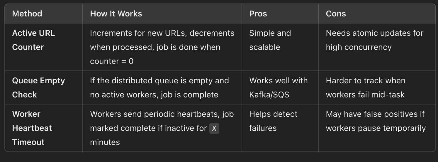
Best Approach?

• Combination of Active URL Counter + Queue Empty Check for real-time accuracy.

• Worker Heartbeat as a backup to detect failures.

• Final cleanup job to verify the job completion status.

Summary

Scaling a web scraping system requires distributed processing, efficient storage, and real-time job tracking. By combining Kafka for buffering, Redis for deduplication, and S3 for scalable storage, we can process millions of URLs per minute efficiently. 🚀

• 📢 Follow for more deep dives on distributed systems!